Enterprise-scale Firewall Decision Trees
One of my highlight projects at Bloomberg was building a tool to conduct contextual firewall policy comparison. I ended up modifying the construction algorithm for an existing data structure, the firewall decision tree, for it to efficiently process enterprise-scale policies. This is a generalized overview of my work starting with an overview of the domain, terminology, and problem. Then, I go over various approaches culminating in the most efficient solution. A discussion of solution pitfalls and further work concludes this post.
A brief primer on firewall policies
Definition and representation
Firewall policies are collections of rules that state what action to take for certain flows. A flow is a 5-tuple consisting
of (source, destination, protocol, source-port, destination-port) and some examples of actions are allow and block.
I will use CIDR notation for the source and destination IPs/subnets.
Most policy rules do not contain source ports, so I will omit them in examples, instead writing a 4-tuple
(source, destination, protocol, destination-port).
An example of a rule:
(1.1.1.0/24, 2.2.2.0/24, tcp, 80) block
This rule blocks traffic from 1.1.1.0/24 to 2.2.2.0/24 on tcp-80, i.e. http.
Usually, to declare rules more efficiently, groups are defined, but no matter how rules are represented, they can be broken down into simple 5-tuples. For example, the composite rule
([1.1.1.0/24, 3.3.3.3], 2.2.2.0/24, tcp, [80, 443]) block, which means block http and https traffic from
1.1.1.0/24 and 3.3.3.3 to 2.2.2.0/24 can be broken down into four simple rules:
(1.1.1.0/24, 2.2.2.0/24, tcp, 80) block
(1.1.1.0/24, 2.2.2.0/24, tcp, 443) block
(3.3.3.3, 2.2.2.0/24, tcp, 80) block
(3.3.3.3, 2.2.2.0/24, tcp, 443) block
Breaking down composite rules into simple rules can be done via Cartesian product:
\(sources \times destinations \times protocols \times destination\_ports\).
Processing
Firewall rules are processed in order for matches. When a packet/flow comes in the first matching rule decides what action to take.
For example, for the set of rules in the previous example the flow (1.1.1.1, 2.2.2.2, tcp, 443) will be matched by the 2nd rule:
(1.1.1.0/24, 2.2.2.0/24, tcp, 443) block, so the flow will be blocked.
Problem
A consequence of the rules being processed in order are shadowing. Shadowing is a form of redundancy when one rule partially or fully overlaps the flows of another rule.
An example of shadowing:
(1.1.1.0/24, 2.2.2.0/24, tcp, 80) allow
(1.1.1.1, 2.2.2.2, tcp, 80) block
Packets destined to 2.2.2.2 from 1.1.1.1 on tcp-80 will be allowed despite rule 2 stating they should be blocked because that flow will be matched by rule 1.
For the shadowing of one rule by another to occur there has to be an intersection between each of the fields for the two rules, so the following example will not cause shadowing since the d-ports are different:
(1.1.1.0/24, 2.2.2.0/24, tcp, 80) allow
(1.1.1.1, 2.2.2.2, tcp, 443) block
Shadowing can cause unintended changes when adding/removing/changing rules in a policy as the true effects of the change depend on the rule’s position and may not be visible via a surface-level comparison, especially when there are tens of thousands of rules, whose flow values may be abstracted behind objects with names, which is common to make rule management more understandable and intentful. Deleting a rule seems like a simple operation, but it may uninentionally expose the flows below it. Similarly, adding a rule may not only be ineffective if that rule is shadowed by preceding rules, it too can uninentionally shadow rules unless it is appended at the end of the list of rules.
A second consequence of shadowing is unoptimized policy, and as the number of rules grows longer it not only makes managing the policy cumbersome and more error-prone, but the policy size may exceed the storage capacity of some equipment like TCAMs, which have very limited storage capacity to maintain packet-processing speed.
Implementing a tool to do a flow comparison betwen two policies and return the set of unshadowed flows present in both policies, whose actions differ across the policies, is the subject of the solution.
Solution
The task of comparing two policies comprises two steps:
a. Comparing intersecting flows between the policies for differences in action
b. Reducing the differing flows to only unshadowed ones
These steps need not be completed in this order; step b) can precede step a) by first reducing the set of flows for each policy to unshadowed only and then comparing these flows with each other.
A naive approach
Implementation
An intuitive approach to attaining the list of unshadowed flows for a policy is to start with an empty set of unshadowed flows, iterate over each rule in order, and subtract the set of unshadowed flows from the flows of this rule. The resulting flows can be added to the set of unshadowed flows.
The time complexity of this solution is \(O(N^2)\) in the total number of flows. For each rule, we subtract at most \(N\) flows.
For two interscting flows, subtracting one flow from another involves subtracting the source CIDRs and destination CIDRs. CIDR subtraction is a time-consuming bit operation, which can yield more disjoint CIDRs than started with, the product of which yields more flows.
As an example, consider subtracting the flows (protocol, port omitted): (1.1.1.0/30, 1.1.10/30) and (1.1.1.1, 1.1.1.1).
(1.1.1.0/30, 1.1.1.0/30) - (1.1.1.1, 1.1.1.1) = (1.1.1.0, 1.1.1.0/30), (1.1.1.1, 1.1.1.0), (1.1.1.1, 1.1.1.2/31), (1.1.1.2/31, 1.1.1.0/30).
The subtraction of two flows resulted in four new disjoint flows. The problem size expands rapdidly with each successive subtraction.
Improvements
There are several improvements we can make for each rule to improve the performance of this apprach.
Instead of subtracting all unshadowed flows from the current rule’s flow, some of which do not overlap with the flow, we can prune this set beforehand. We achieve this by using radix trees to store the unshadowed sources and destinations. This way instead of linearly scanning all the flows, we can narrow down the overlapping sources and destinations in \(log(N)\) time.
Since we must also consider that the protocols and d-ports overlap, we can bucket the flows by (protocol, d-port) pair, all flows for one (protocol, d-port) being in the same bucket. Now, for a given rule flow we only need to process the flows in the flow’s (protocol, d-port) bucket [if such a bucket exists]. And of those flows, we only need to subtract the ones, whose sources and destinations overlap with the given flow’s sources and destinations, which we find using the radix trees.
The amount of CIDR subtraction done for each flow is greatly reduced with these methods and there is an added benefit of allowing parallelization. Previously, since each rule’s unshadowed flows depended on the preceding flows, we could not parallelize the work, but, now, we can bucket all rule flows by (protocol, d-port) in advance and then process all of the buckets in parallel since there is no overlap between buckets. The rule flows within a bucket must still be processed synchronously.
Unfortunately, the above methods do not improve the asymptotic runtime of the solution and do not reduce enterprise policy
processing time enough for practical use. One simple worst-case scenario that occurs frequently is the rule flow
(0.0.0.0/0, 0.0.0.0/0, all, all). This usually appears at the end of a policy, the final “default drop” rule. This flow
overlaps with every flow and since it is at the end we must subtract all the unshadowed flows from it. This single operation
takes an impractical amount of time to seriously consider this solution.
Using firewall decision trees
Original structure and algorithms
To solve this problem I conducted an extensive literature review for existing solutions. A series of papers (Liu and Gouda 1237) described a data structure called the firewall decision tree [FDT], which had several uses:
- Policy comparison
- Policy optimization (shadowing analysis)
- Policy testing (more efficient flow matching and coverage analysis)
This was a promising approach with benefits beyond solving this problem.
Using the FDT for policy comparison described in the paper:
- Construct an FDT for each policy
- Find differing flows between the policies by merging the constructed FDTs
The FDT construction process removes shadowed flows. It is more efficient than the aforementioned naive approach. The key to
its efficiency is representing the fields of a flow as numeric intervals, [start, end] (Liu and Gouda 1241).
Instead of representing sources and destinations as CIDRs, they are represented as numerical intervals in the range 0-2^32.
Protocols can be represented numerically in the range 0-255 via this mapping.
Finally, ports are numbers in the range 0-2^16.
The example flow (1.1.1.0/24, 2.2.2.0/24, tcp, 80) becomes ([16843008, 16843263], [33686016, 33686271], 16, 80).
Interval subtraction is less costly than CIDR subtraction. Indeed, no arithmetic or bit manipulation is needed to subtract two intervals:
[1, 10] - [2, 4] = [1, 1], [5, 10]. For a set of overlapping intervals, we can use this algorithm
to merge them while removing overlaps. The runtime complexity is \(O(NlogN)\) in the number of intervals.
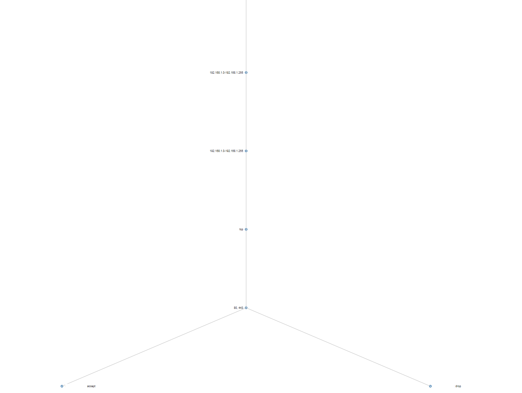
The result of the construction algorithm is a tree whose levels comprise flow field intervals, i.e. level 1 is source intervals, level 2 is destination intervals, level 3 is protocol intervals, and level 4 is destination port intervals. At the end of each tree path is an action, so the actions can be considered the last level and they make up the leaves of the tree. Hence, every path of the tree is a flow, and the total number of unshadowed flows is equal to the number of paths/leaves of the tree.
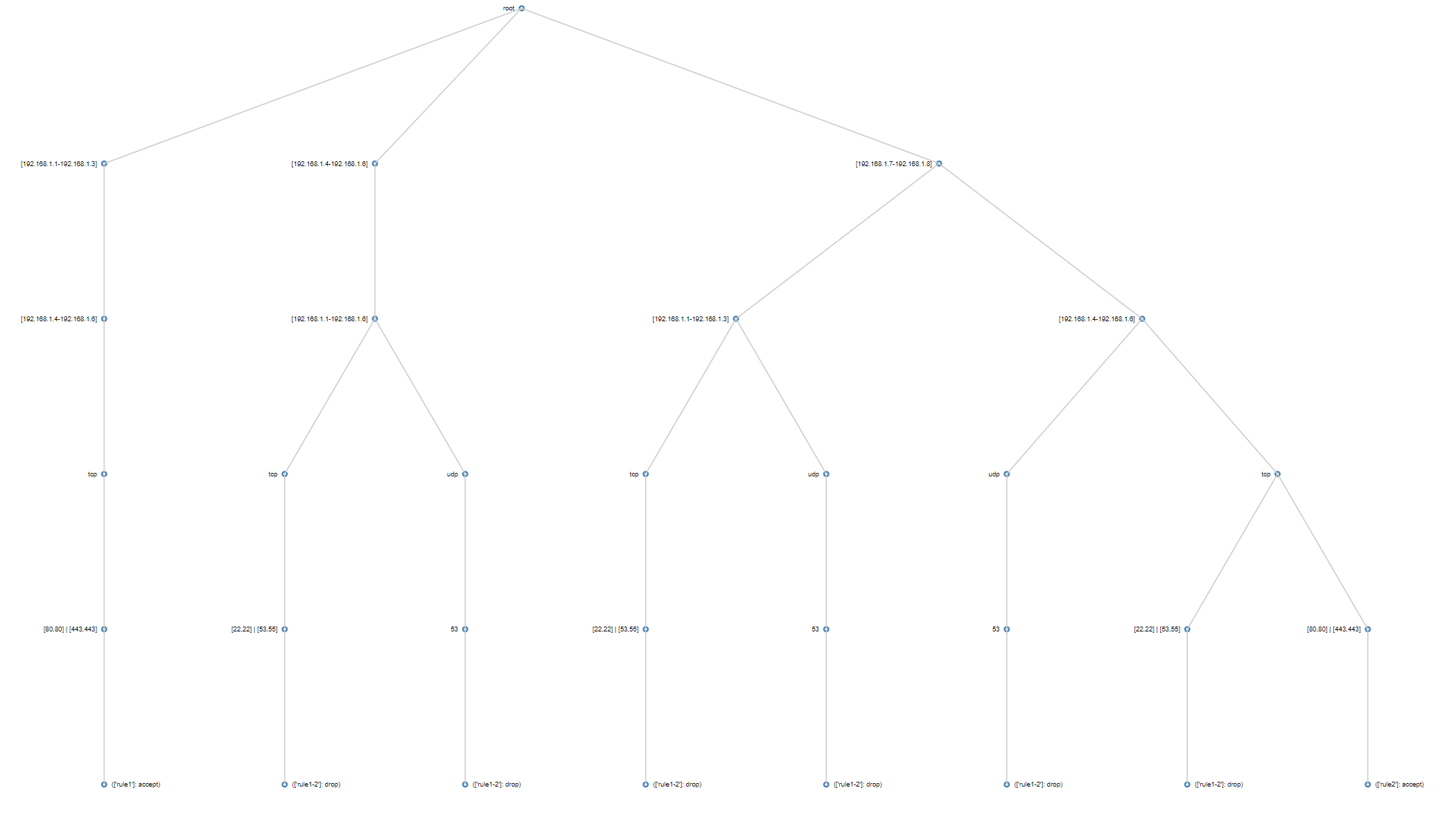 A visual representation of a firewall decision tree. Internally protocols are stored as numeric intervals with equal start and end.
The construction is described on page 1243 of Liu and Gouda, but I have abridged it here:
- Append each rule flow in order into the tree. Start from the tree’s root level of source intervals.
- Merge flow’s intervals with overlapping tree’s intervals and create nodes for the resulting disjoint intervals accordingly.
- Copy old interval subtrees to new interval nodes.
- Proceed to the children (next level) of interval nodes covered by the flow’s intervals.
- Repeat steps 2-3 until entire flow is merged.
Once FDTs for both policies are constructed, the paper describes the comparison algorithm, which consists of making the trees isomorphic to each other to make them comparable. Essentially, at the end of this process, all the flows in one tree exist in the other with potentially a different action (so, in fact, the trees are semi-isomoprhic). It is then a matter of iterating over all the flows to find ones with differing actions (Liu and Gouda 1245).
There are several pitfalls to this algorithm in its current state:
- Deep copying subtrees is time-consuming.
- Constructing an FDT for each policy and then shaping them to be semi-isomorphic is time-consuming.
- There is no room for parallelization in FDT construction due to the synchronous [appending new paths to the tree] nature of the construction algorithm.
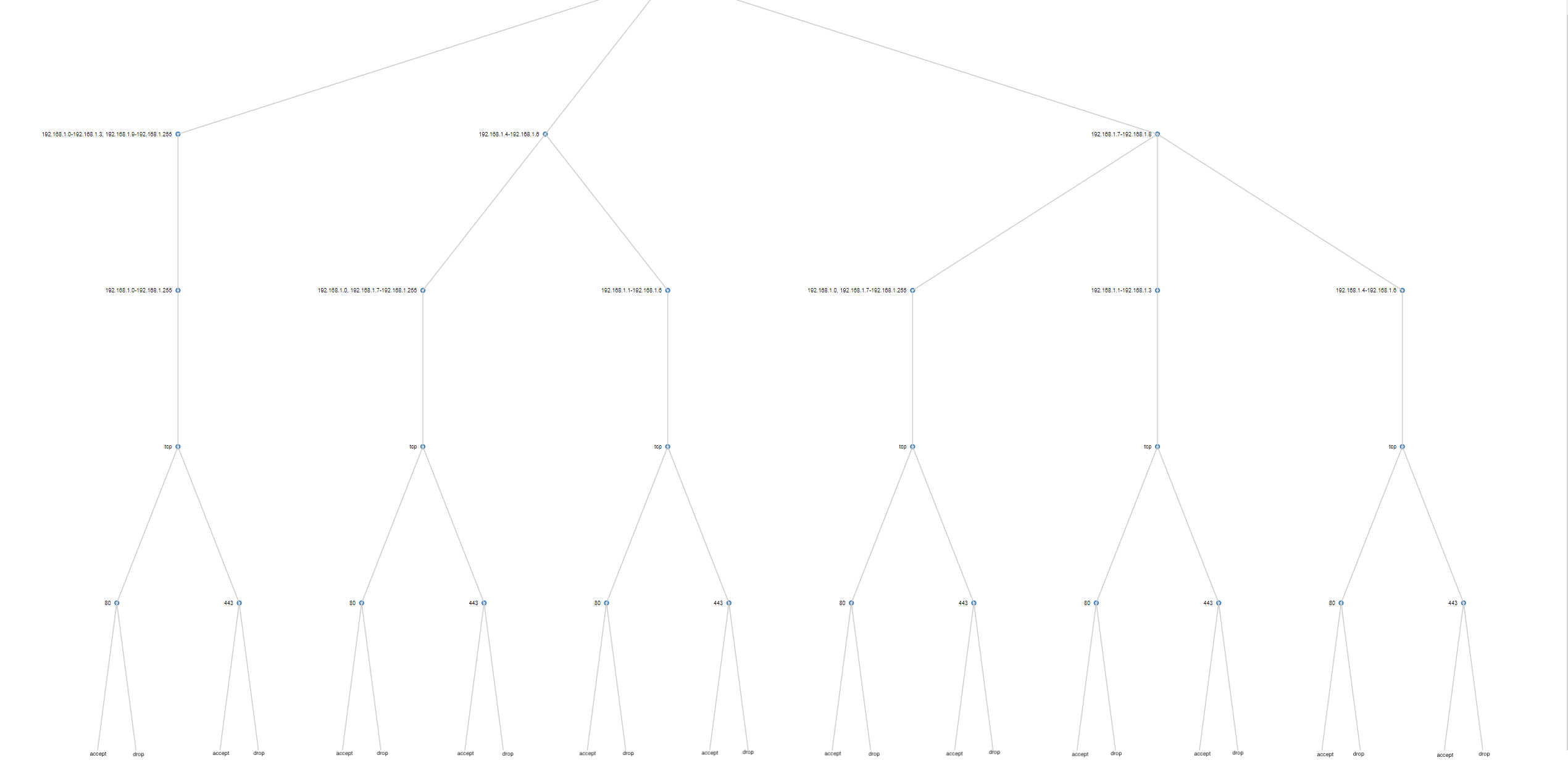
 Vertical construction algorithm for a firewall policy. Compare with horizontal below.
Even though the overall efficiency of this solution is superior to the naive method present above (complexity analysis can be found at Liu and Gouda 1247), the policies it was benchmarked on (Liu and Gouda 1249) have orders of magnitude fewer rules than the enterprise policies I was working with, so I needed to rethink portions of the algorithm to improve performance.
New modifications to improve performance
My contribution to the solution was redesigning the implementation of this method to avoid any copying, avoid making the trees isomorphic to each other altogether, and utilize parallelization.
Modification 1: Instead of constructing two FDTs, one for each policy, and then making them isomorphic to each other, I immediately construct a combined tree that includes the flows of both policies. In this tree, flows have two action leaves, one from each policy. If only one of the policies contains a flow, the other action is empty. Since the construction algorithm is responsible for the majority of the runtime, this signficantly improves performance and space.
Modification 2: Instead of following a vertical construction approach of merging one flow after another to the tree, I use a horizontal level-based approach. I merge all the source intervals of all the flows first, then, for each source interval, merge all the destination intervals, then protocols, then ports. This simultaneously avoids subtree copying and opens up the potential to parallelize.
 Horizontal construction algorithm for the same policy. Compare with vertical above.
The result of the construction algorithm is a tree, whose differing flows are trivial to find by iterating over all flows to filter ones with more than one action leaf and whose actions differ.
Further speed enhancements can be made by parallelizing construction and storing interval merging results in a cache so as not to solve the same interval merging problem more than once because intervals are often repeated, especially for protocols and ports, both of which have small sets of commonly used values. Target protocols in policy rules are typically tcp (6), udp (17), and icmp (1) and target ports are http (80), https (443), and dns (53). These auxiliary changes prove effective in practice.
| Method | Sources | Destinations | Protocols | Ports | Total |
|---|---|---|---|---|---|
| serial | 0.07 | 8.87 | 0.86 | 4.38 | 14.18 |
| targeted parallel | 0.07 | 1.07 (parallel) | 0.86 | 4.38 | 6.38 |
| parallel and cache | 0.07 | 1.07 (parallel) | 0.86 | 1.19 (cache) | 3.19 |
A summary of FDT + speed enhancements performance on an enterprise policy with ~100,000 rules [results in minutes].
Simplifying the tree
Merging overlapping intervals during the construction process can make the flows overly granular. Presenting results is then cumbersome and the firewall decision tree takes up more space than necessary.
 A tree with 24 flows even though all of the flows can be encapsulated by 2 flows with unions of intervals.
To simplify the reporting of differing flows and structure of the tree, we can union interval nodes whose subtrees are the same. Starting at the bottom of the tree at the port level, if two port nodes have the same action leaves, we can union the ports into one combined port node. Advancing up the tree to the protocol level, we check if any protocol nodes have equal subtrees, in which case we union them. We continue in this manner all the way up to the tree root. The idea of comparing child contents in this process is inspired by how Merkle trees work. The runtime complexity of this simplification algorithm is \(O(N)\) where \(N\) is the number of nodes in the tree since we visit each node once.
The result is a simpler, more understandale set of flows.
 After simplification, the above tree reduces to 2 flows.
Discussion and further work
The described modifications to the firewall decision tree construction algorithm significantly improve performance and space. They enable parallelization through level-based construction and simplify the presentation of results. These enhancements make it feasible to conduct contextual firewall policy comparison at a massive scale.
A consequence of building a tree from the rules of multiple policies as described is that this process supports more than two policies. In fact, each port node can have as many action leaves as there are policies, and the algorithm simply works. The other aforementioned benefits of using firewall decision trees are maintained as well.
Further speed improvements could be made by preprocessing the flows before tree construction and splitting by (protocol, d-port) combo as mentioned in the improvements for the naive implementation. Another approach to consider is merging overlapping intervals for each field and then connecting intervals to their children to construct the levels of the tree.